Ecommerce merchandising: test your product-position assumptions
A historical ten-book experiment shows how a simple placement adjustment can miss parts of the pattern, and how to test that assumption before comparing product cards.
Original reanalysis of the released 2024 book-choice experiment by Compiani, Morozov and Seiler.
Abstract
Before deciding that one offer is stronger than another, a business needs to consider where each appeared. We used a released 2024 experiment with ten e-books to test two ways of accounting for position. Allowing each position its own adjustment predicted choices better overall than applying the same adjustment for every step down the list. It was less accurate at some individual positions, so the complete comparison matters.
Both models used the same book and price information. We fitted them on 6,176 participants and checked their predictions on 3,088 other participants. The choices were hypothetical, and everyone had to select a book. For businesses and creators comparing product cards, the lesson is to test placement assumptions before attributing results to an offer. The study does not estimate a sales increase or identify the best product order.
Suppose the product at the top of a page gets the most clicks. Is it a stronger offer, or did its place in the list help? A business needs a useful answer before it rewrites the other cards, discounts the weaker-looking items or changes the assortment.
Accounting for position sounds straightforward until you ask how. Should each move down the list receive the same adjustment? We used a historical experiment to compare that simple approach with a more flexible one, then tested both on participants kept out of model fitting.
The same products, different positions

What should a product-position comparison tell you?
A product-card comparison should help you separate the item being offered from the way it was presented. If one product usually appears first and another usually appears last, their totals alone do not answer whether shoppers prefer one offer.
The simple approach we test gives every step down the list the same adjustment to the model’s underlying preference score. The useful question is whether it predicts choices well enough, compared with allowing different positions to have different adjustments.
We tested those two approaches using a released book-choice experiment. The result is relevant to businesses and creators comparing products on a collection page or digital storefront. It supplies a way to examine a measurement assumption, rather than a rule for where to put your best-selling item.
This matters when an offer appears in more than one place. A creator might feature the same download in a collection and a launch page. A retailer might change the order of a category list. The item, price, audience and presentation can differ together. A position adjustment is an assumption about part of that comparison, and it deserves its own check.
What did people choose in the book experiment?
Giovanni Compiani, Ilya Morozov and Stephan Seiler asked Prolific recruits to make hypothetical choices from ten e-books, with randomized order and prices. Participants had to select a book; there was no option to buy nothing. We use the first task within each retained submission, not the later task that removed the chosen book.[1]
The authors already report responses to rank and price. Their wider research studies how text and images help estimate product substitution. Our question is narrower: does replacing a single position term improve prediction for participants whose choices were kept out of model fitting?
Following the original eligibility rules leaves 9,265 submissions with 9,264 distinct Prolific participant IDs. One ID appears twice. We keep both submissions together and give that participant the same total weight as every other participant. A submission is not automatically a separate person, and a first task is not necessarily that person’s first exposure to the experiment.[2][3]
The retained source dates run from June 11 to June 26, 2024. The manuscript describes June 14–27, so we disclose the difference and apply no date exclusion. Country and age eligibility were not established in the reviewed materials; these are not estimates for U.S. shoppers or another national population.[1][2]
The participant stays together throughout the comparison
Selected first-task submissions after the original author eligibility rules; dates in retained source records June 11–26, 2024.
| Group | Participants (by platform ID) | Retained submissions |
|---|---|---|
| All retained | 9,264 | 9,265 |
| Training | 6,176 | 6,176 |
| Held out for evaluation | 3,088 | 3,089 |
Which position model predicted held-out choices better?
The flexible position model predicted held-out choices better on the prespecified scoring measure. Both models account for which book was offered and its displayed price. They differ only in how they represent position.
The baseline uses one coefficient for each step down the list. The flexible model uses separate adjustments for positions two through ten, relative to the first. That gives it more freedom, but also more parameters to estimate. Better fit to its own training data would not, by itself, settle the comparison.
We therefore fitted both models using 6,176 participants and evaluated them on the other 3,088 participants. Every submission from a participant stayed on the same side of that split. The test group contains 3,089 submissions because it includes the repeated participant.
To compare predictions, we used a negative log score. A model receives a smaller penalty when it assigns more probability to the choice a person actually makes. It receives a larger penalty when it assigns very little probability to that choice. Lower average negative log scores are better.
The held-out average was 2.2260 for the baseline and 2.2154 for the flexible model, in natural-log units, also called nats. These are prediction scores, not percentages of correct answers. Training and test scores are shown together so the comparison does not rely on the easier task of describing data the model has already seen.
Two models, evaluated on the same participants
Selected 2024 ten-book first-task choices. Training: 6,176 participants and submissions. Test: 3,088 participants and 3,089 submissions.
| Position model | Training score (nats) | Held-out score (nats) |
|---|---|---|
| One linear position term | 2.2046 | 2.2260 |
| Separate position terms | 2.1899 | 2.2154 |
The paired improvement was 0.0106 nats per participant, with an approximate 95% interval from 0.0044 to 0.0168. Here, a positive improvement favors the flexible model. The result is small on this scoring scale, but the interval lies above zero.[4]
This interval treats the two fitted models as fixed and assumes independent participant groups. It does not include uncertainty from fitting the models on another training sample. The finding supports a predictive improvement in this selected historical task; it does not turn the score difference into a sales increase.
The flexible model improves the held-out log score
Paired comparison among 3,088 test participants in the selected historical ten-book task.
| Comparison | Improvement (nats) | 95% interval: lower (nats) | 95% interval: upper (nats) |
|---|---|---|---|
| Flexible minus baseline log score | 0.0106 | 0.0044 | 0.0168 |
Where did the two models miss the observed choices?
The complete position comparison shows why the overall score should come with detail. For each position, we compare its observed choice share with the average probability assigned by each model. These are equal-participant averages in the held-out group, not click-through rates.
At position one, the observed share was 17.16%. The baseline predicted 14.64%, while the flexible model predicted 17.73%. At position ten, the observed share was 9.18%, compared with predictions of 6.37% and 8.74%. The flexible model was closer at both ends of this particular list.
Observed and predicted choices at all ten positions
Held-out group: 3,088 participants and 3,089 first-task submissions from the released 2024 experiment.
| Position | Observed choice share | Baseline mean probability | Flexible mean probability | Chosen submissions |
|---|---|---|---|---|
| Position 1 | 17.16% | 14.64% | 17.73% | 530 |
| Position 2 | 13.60% | 13.20% | 14.84% | 420 |
| Position 3 | 9.91% | 12.06% | 9.74% | 306 |
| Position 4 | 10.91% | 11.21% | 9.26% | 337 |
| Position 5 | 9.20% | 10.09% | 8.94% | 284 |
| Position 6 | 7.08% | 9.25% | 8.01% | 219 |
| Position 7 | 8.00% | 8.44% | 7.57% | 247 |
| Position 8 | 7.12% | 7.67% | 7.47% | 220 |
| Position 9 | 7.84% | 7.08% | 7.69% | 242 |
| Position 10 | 9.18% | 6.37% | 8.74% | 284 |
The flexible model was not closer everywhere. At position four, the observed share was 10.91%. The baseline predicted 11.21%, while the flexible model predicted 9.26%. The extra flexibility improved the overall held-out score while leaving a larger discrepancy at that position.
The next table shows observed minus predicted shares. A positive gap means the model predicted too little choice at that position; a negative gap means it predicted too much. Keeping all ten positions visible prevents a good-looking endpoint from standing in for the whole comparison.
Both models’ gaps from the observed choices
Observed choice share minus mean predicted probability for each of the ten positions, using the same 3,088 test participants.
| Position | Observed minus baseline | Observed minus flexible |
|---|---|---|
| Position 1 | 2.52 percentage points | -0.57 percentage points |
| Position 2 | 0.41 percentage points | -1.24 percentage points |
| Position 3 | -2.15 percentage points | 0.17 percentage points |
| Position 4 | -0.29 percentage points | 1.65 percentage points |
| Position 5 | -0.89 percentage points | 0.26 percentage points |
| Position 6 | -2.17 percentage points | -0.93 percentage points |
| Position 7 | -0.44 percentage points | 0.43 percentage points |
| Position 8 | -0.55 percentage points | -0.35 percentage points |
| Position 9 | 0.76 percentage points | 0.14 percentage points |
| Position 10 | 2.81 percentage points | 0.44 percentage points |
These position rows are descriptive, with no separate significance claims. The experiment did not measure eye movements or attention, and this analysis does not identify why a position differs. Nor does a curved pattern of observed shares, on its own, refute the baseline: its position term is linear in the model’s underlying preference score, not in choice percentages.
Simply subtracting the first and last observed shares would answer a different question. Those shares summarize choices across products and prices. Both fitted models account for book identity and price before assigning probabilities across the ten options. Neither the endpoint difference nor the model comparison tells you what would happen if you moved a particular product on a live store.
A product-position measurement template you can use
Before comparing offers, write a short measurement brief. The following template is ungated and illustrative. It applies the study’s lesson about checking assumptions; it does not promise that the same model will suit your storefront.
Decision: “We need to decide [which product comparison or presentation change] for [page or campaign] during [period].” Name the decision before choosing a favorable metric.
Outcome: “We will measure [choice, click, add-to-cart or purchase].” Select the outcome your records actually support. Keep the offered alternatives, their order and displayed prices alongside it. A forced-choice result should remain separate from a purchase result.
Unit: “Our unit is [participant or another clearly defined unit]. Repeat visits or submissions will be handled by [rule].” Keep the same person’s observations together when evaluating prediction for new people. Do not treat an anonymous session identifier as proof of a unique person.
Comparison: “Both models will use the same products, price information and eligible observations. They will differ in [the position assumption].” Specify the simple alternative as well as the more flexible one.
Evaluation: “We will reserve [a defined group] before fitting and compare [a named scoring measure]. We will show all positions.” Decide how to report an unresolved or worse result before seeing it.
Use: “This result will inform [measurement decision]. Evidence about [commercial outcome not measured here] is still needed before [commercial decision].” This last sentence keeps a prediction exercise from quietly becoming a revenue forecast.
Keep the same participant on one side of the test
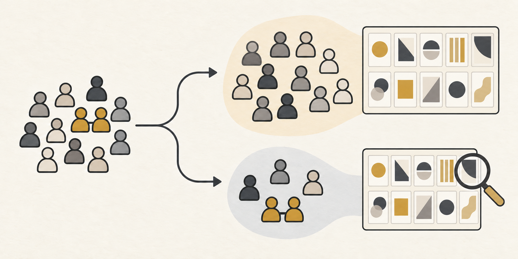
Define the comparison
Name the product, position, outcome and observation unit.
Reserve the evaluation group
Keep each participant’s submissions together.
Check the complete result
Compare predictions and show every position, including worse results.
A worked example: a creator comparing digital offers
Consider a fictional creator selling a writing workbook, a workshop and a bundle. The bundle appears at the top of a launch page and receives the most clicks. The creator is considering rewriting the other product descriptions.
The measurement brief changes the immediate question. The observed outcome is a click, not a sale. The available records need to show which offers were displayed, in what order and at what prices. If the bundle always occupies the first slot, those records cannot cleanly separate that bundle from that position.
The creator’s completed brief could read: “We want to know whether our way of accounting for position predicts clicks from new visitors. We will compare the same offers and price information, keep repeat observations together, and report the full position comparison. We will make no claim about purchases from click records.” This is a fictional example of a measurement question, not a proposed result.
A sensible next step is to plan a comparison with enough variation to distinguish product and position, while retaining the same outcome definition. The creator could then compare a simple position adjustment with a more flexible one on a reserved group. This would be a new study of that page; the book experiment supplies no expected click rate for it.
If the flexible approach predicts the reserved group better, the creator has a reason to revisit how the report accounts for placement. That still does not show that moving the bundle will increase revenue. A commercial decision would require evidence on the actual presentation change and the outcome that matters to the business.
If the comparison is unresolved, the creator should say so. Additional flexibility is not automatically a better business tool. The practical gain is a clearer sequence: understand what the records can separate, test the measurement assumption, then decide whether another experiment is needed.
How did Influence IQ calculate the comparison?
We used the authors’ edited response release and original selection rules. The first 553 pilot or test records are excluded by their fixed file position. The remaining frame contains 10,775 submissions. The comprehension filters leave 9,344; the completion filter leaves 9,265.[2]
Consent, finished-status and the minimum 60-second duration rule remove no additional submissions at their respective steps. Completion and duration are post-exposure filters, so the retained group is a selected sample.
Prolific participant IDs define the groups. A deterministic hash split assigns two-thirds of the groups to training and the rest to test, without using their choices. Within each group, every retained first-task submission shares that participant’s contribution equally. The same weighting applies to fitting, scoring and the position tables.[3]
Both models are unpenalized multinomial logits with nine book indicators and one linear price term. The baseline adds one linear position term, for 11 parameters. The flexible model adds nine position indicators, for 19. Position one and the numerically smallest product ID provide the reference categories. All eligible choice sets contain the same ten products, with selected ID, price and position checked for agreement.
We fit the models on the training group, retain the fitted coefficients, and then score the test choices. The interval uses the standard deviation of the paired participant score differences, 3,088 participant units and 3,087 degrees of freedom. It is an approximate Student-t interval except under its exact normal-score assumptions. All ten position comparisons remain descriptive.[4]
The baseline’s primary optimizer returned a numerical warning. It still met every accuracy condition specified before fitting, including a second-start comparison. We retained that original fit; the detailed diagnostics are included with the reproduction materials.[5]
The downloads provide the displayed results, original analysis code and aggregate numerical output. They exclude source response rows, participant IDs and book artwork. Obtain the source data separately from the authors’ release. Influence IQ is responsible for this reanalysis and its interpretation.
The CSV uses this page’s language. The package contains original calculation code, English method documentation and aggregate results. Source response rows and book assets are not included; obtain the data separately from the authors’ release.
Sources and notes
- Compiani, Morozov and Seiler, Demand Estimation with Text and Image Data, manuscript version 4, February 17, 2026, Section 3 and Appendix C. The authors already study responses to rank and price. Our held-out participant comparison is an original, narrower reanalysis.
- Authors’ DeepLogitReplication release at commit 8c4f37a58c3a5049d3dff8ad171235b2c6ef01ec. We follow the edited response file’s original positional pilot cutoff and author eligibility rules. Retained source dates are June 11–26, 2024, differing from the manuscript’s June 14–27 description; dates do not determine inclusion.
- Prolific distinguishes a participant ID from a study or submission identifier. We preserve the exact participant IDs for grouping. These IDs do not independently verify that each ID represents a different person or establish that a retained submission was that person’s first exposure.
- Influence IQ’s prespecified comparison averages the flexible-minus-baseline log probability within each test participant, then across participants. The 95% interval is the mean plus or minus the Student-t critical value times the participant standard deviation divided by the square root of 3,088. It assumes independent participant groups, conditions on fixed training fits and excludes training-fit uncertainty; exactness requires identically distributed normal participant differences with common variance.
- The baseline zero-start fit returned a precision warning. Its maximum absolute mean gradient was 3.12×10⁻⁹, Newton decrement 2.50×10⁻⁸ and maximum two-start log-probability difference 7.46×10⁻⁸, below the prespecified limits 10⁻⁸, 10⁻⁶ and 10⁻⁷. Both models also met the positive-curvature and objective-agreement conditions. The primary zero-start coefficients were retained.
This English article is the source version. Language versions describe the same historical experiment; they are not country-specific shopping estimates.